HFSCREEN and LTHOMAS

 HFSCREEN = real    (truncate the long range Fock potential)

In combination with PBE potentials, attributing a value to HFSCREEN will switch from the PBE0 functional (in case LHFCALC=.TRUE.) to the closely related HSE03 or HSE06 functional [67,68,69].

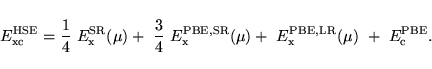
The HSE03 and HSE06 functional replaces the slowly decaying long-ranged part of the Fock exchange, by the corresponding density functional counterpart. The resulting expression for the exchange-correlation energy is given by:

$$E_{\mathrm{xc}}^{\mathrm{HSE}}= \frac{1}{4}~E_{\mathrm{x}}^{... ...rm{x}}^{\mathrm{PBE,LR}}(\mu)~+~E_{\mathrm{c}}^{\mathrm{PBE}}.$$ (25)

As can be seen above, the separation of the electron-electron interaction into a short- and long-ranged part, labeled SR and LR respectively, is realized only in the exchange interactions. Electronic correlation is represented by the corresponding part of the PBE density functional.

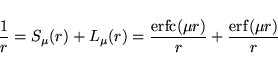
The decomposition of the Coulomb kernel is obtained using the following construction ($\mu\equiv$ HFSCREEN):

$$\frac{1}{r}=S_{\mu}(r)+L_{\mu}(r)=\frac{{\rm erfc}(\mu r)}{r}+\frac{{\rm erf} (\mu r)}{r}$$ (26)

where $r=\vert{\bf r}-{\bf r}'\vert$, and $\mu$ is the parameter that defines the range-separation, and is related to a characteristic distance, ($2/\mu$), at which the short-range interactions become negligible.

Note: It has been shown [67] that the optimum $\mu$, controlling the range separation is approximately $0.2-0.3$ Å$^{-1}$. To conform with the HSE06 functional you need to select ( HFSCREEN=0.2) [67,68,69].

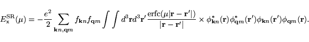
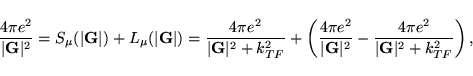
Using the decomposed Coulomb kernel and Equ. (6.13), one straightforwardly obtains:

$$E^{\rm SR}_{\rm x}(\mu)= -\frac{e^2}{2}\sum_{{\bf k}n,{\bf q... ...}({\bf r}') \phi_{{\bf k}n}({\bf r}')\phi_{{\bf q}m}({\bf r}).$$ (27)

The representation of the corresponding short-ranged Fock potential in reciprocal space is given by

$$V^{\rm SR}_{\bf k}\left( {\bf G},{\bf G}'\right) = \langle {\bf k}+{\bf G} \vert V^{\rm SR}_x [\mu] \vert {\bf k}+{\bf G}'\rangle$$

$$= -\frac{4\pi e^2}{\Omega} \sum_{m{\bf q}}f_{{\bf q}m}\sum_{{\bf G}... ...t^2} \times \left( 1-e^{-\vert{\bf k}-{\bf q}+{\bf G}''\vert^2 /4\mu^2} \right)$$ (28)

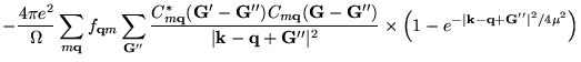
Clearly, the only difference to the reciprocal space representation of the complete (undecomposed) Fock exchange potential, given by Equ. (6.17), is the second factor in the summand in Equ. (6.22), representing the complementary error function in reciprocal space.

The short-ranged PBE exchange energy and potential, and their long-ranged counterparts, are arrived at using the same decomposition [Equ. (6.20)], in accordance with Heyd et al. [67] It is easily seen from Equ. (6.20) that the long-range term becomes zero for $\mu=0$, and the short-range contribution then equals the full Coulomb operator, whereas for $\mu \to \infty$ it is the other way around. Consequently, the two limiting cases of the HSE03/HSE06 functional [see Equ. (6.19)] are a true PBE0 functional for $\mu=0$, and a pure PBE calculation for $\mu \to \infty$.

Note: A comprehensive study of the performance of the HSE03/HSE06 functional compared to the PBE and PBE0 functionals can be found in Ref. [73]. The B3LYP functional was investigated in Ref. [74]. Further applications of hybrid functionals to selected materials can be found in the following references: Ceria (Ref. [75]), lead chalcogenides (Ref. [76]), CO adsorption on metals (Refs. [77,78]), defects in ZnO (Ref. [79]), excitonic properties (Ref. [80]), SrTiO$_3$ and BaTiO$_3$ (Ref. [81]).

LTHOMAS

If the flag LTHOMAS is set, a similar decomposition of the exchange functional into a long range and a short range part is used. This time, it is more convenient to write the decomposition in reciprocal space:

$$\frac{4 \pi e^2}{\vert{\bf G}\vert^2}=S_{\mu}(\vert{\bf G}\v... ...t^2} -\frac{4 \pi e^2}{\vert{\bf G}\vert^2 +k_{TF}^2} \right),$$ (29)

where $k_{TF}$ is the Thomas-Fermi screening length. HFSCREEN is used to specify the parameter $k_{TF}$. For typical semi-conductors, the Thomas-Fermi screening length is about 1.8 Å$^{-1}$, and setting HFSCREEN to this value yields reasonable band gaps for most materials. In principle, however, the Thomas-Fermi screening length depends on the valence electron density; VASP determines this parameter from the number of valence electrons (POTCAR) and the volume and writes the corresponding value to the OUTCAR file:

  Thomas-Fermi vector in A             =   2.00000

Since, VASP counts the semi-core states and $d$-states as valence electrons, although these states do not contribute to the screening, the values reported by VASP are, however, often incorrect. Details can be found in literature [70,71,72]. Another important detail concerns that implementation of the density functional part in the screened exchange case. Literature suggests that a global enhancement factor $z$ (see Equ. (3.15) in Ref. [72]) should be used, whereas VASP implements a local density dependent enhancement factor $z= k_{TF}/\bar k$, where $\bar k$ is the Fermi wave vector corresponding to the local density (and not the average density as suggested in Ref. [72]). The VASP implementation is in the spirit of the local density approximation.